A practical engineering view on ventilation, control logic, airflow delivery, and why IAQ data alone does not explain IAQ in commercial buildings
Indoor air quality in buildings is often reduced to one simple idea: if the CO₂ reading stays below a chosen threshold, ventilation must be acceptable.
In practice, the situation is more complex. Real occupied spaces behave dynamically. CO₂ rises with occupancy, responds to airflow with delay, and is strongly influenced by sensor location, reset quality between occupied periods, and the ability of the ventilation system to react while the space is in use.
This article draws on a structured engineering review of an anonymized classroom dataset. The classroom remains the supporting case study, but the lessons are broader. The goal was not to produce another generic IAQ commentary. It was to reorganize raw time-series data into an analysable structure, apply a mass-balance model, test practical operating strategies, and extract useful lessons for ventilation commissioning and building operation more generally.
BAARCH perspective. Good ventilation design is not only about selecting a nominal airflow per person. It is about understanding how the space actually behaves over time: rise, delay, purge, reset, and recovery. That is where engineering judgment matters, whether the space is a classroom, meeting room, office zone, retail unit, or other commercial area.
Although the supporting analysis comes from one classroom, the philosophy is not specific to schools. The same reasoning applies to office meeting rooms, open-plan office zones, retail areas, training rooms, healthcare waiting spaces, and other commercial environments where occupancy varies, ventilation is controlled dynamically, and the difference between measured data and actual airflow performance can be significant.
Why indoor CO₂ should be treated as a dynamic engineering problem
Many ventilation discussions still treat CO₂ as a static compliance number. That approach misses the main operational reality. In a tight occupied zone with low air velocities and limited mixing, the question is not only whether a target such as 1000 ppm is exceeded. The more useful question is when it is exceeded, for how long, how quickly it rises, and whether the space is properly reset before the next occupied period begins.
That distinction matters because occupants do not experience a space as a daily average. They experience it minute by minute. A control strategy can look acceptable on paper and still deliver a poor breathing-zone experience if the signal is delayed, averaged, or poorly interpreted.
- Many commercial spaces have long or back-to-back occupancy blocks.
- Pre-ventilation can improve the starting point without being sufficient during the occupied period itself.
- Return-duct measurements can lag the concentration actually experienced in the occupied zone.
What the dataset contained and how it was structured
The original material came from chart exports combining several heterogeneous time-series blocks. These included mobile CO₂ sensors located in the occupied zone, fixed BMS sensors in the return path, motorized damper positions, schedule data used as an occupancy proxy, and a damper-position-to-airflow calibration table derived from field measurement.
To make the analysis usable, the dataset was reorganized into a clear long-format structure with five main tables:
- IAQ measurements: timestamp, room identifier, sensor type, sensor ID, CO₂ in ppm
- Room schedule: timestamp, room identifier, occupancy level
- Damper position: timestamp, room identifier, damper position in percent
- Airflow calibration: damper position versus airflow in m³/h
- Estimated airflow: timestamp, room identifier, estimated delivered outdoor airflow
All data were aligned on a regular 5-minute time grid to support phase-shift analysis, mass-balance calculation, and operational simulations.
Sensor placement changes what you think the problem is
One of the most important lessons from the analysis is that not all CO₂ measurements represent occupant exposure equally. The dataset combines mobile zone measurements with BMS return-path measurements. That is useful, but it also highlights a common commissioning issue found across many commercial buildings.
In a building with strong airtightness, slow diffusion, and low supply-air velocities, the return-duct or return-path sensor behaves as an integrated signal. It reflects a spatially and temporally mixed value. That makes it useful for system-level monitoring, but not necessarily a direct proxy for what occupants are breathing at that exact moment.
In practical terms, this means the return measurement can show both delay and damping relative to the occupied zone. When a control loop relies too heavily on that delayed signal, the system may react late, then continue ventilating after the peak exposure period has already passed.
Commissioning implication. Return-duct CO₂ is not wrong, but it must be interpreted as a delayed system signal. For occupant experience and detailed tuning, zone measurements remain the reference.
The physical model behind the analysis
The review used a standard single-zone mass-balance formulation for CO₂:
dC/dt = (Q/V) × (Cext − C) + G(t)/V
Indoor concentration depends on outdoor air supply, room volume, outdoor background concentration, and internal generation linked to occupancy and activity. Rather than treat generation as a theoretical constant only, the analysis identified it from the measured CO₂ dynamics and estimated airflow. That made it possible to test practical scenarios such as pre-ventilation, inter-session purge, and required airflow levels for different IAQ targets.
What the baseline actually showed
Under the baseline condition, with average airflow around 450 m³/h, exceedances above 800 ppm were systematic on active sessions, and several sessions exceeded 1000 ppm. The most difficult periods were long morning sessions and a late-afternoon period that started with already elevated CO₂, suggesting insufficient reset between occupancy cycles or residual occupancy effects.
Figure 1. Peak CO₂ by active occupied session in the case-study room
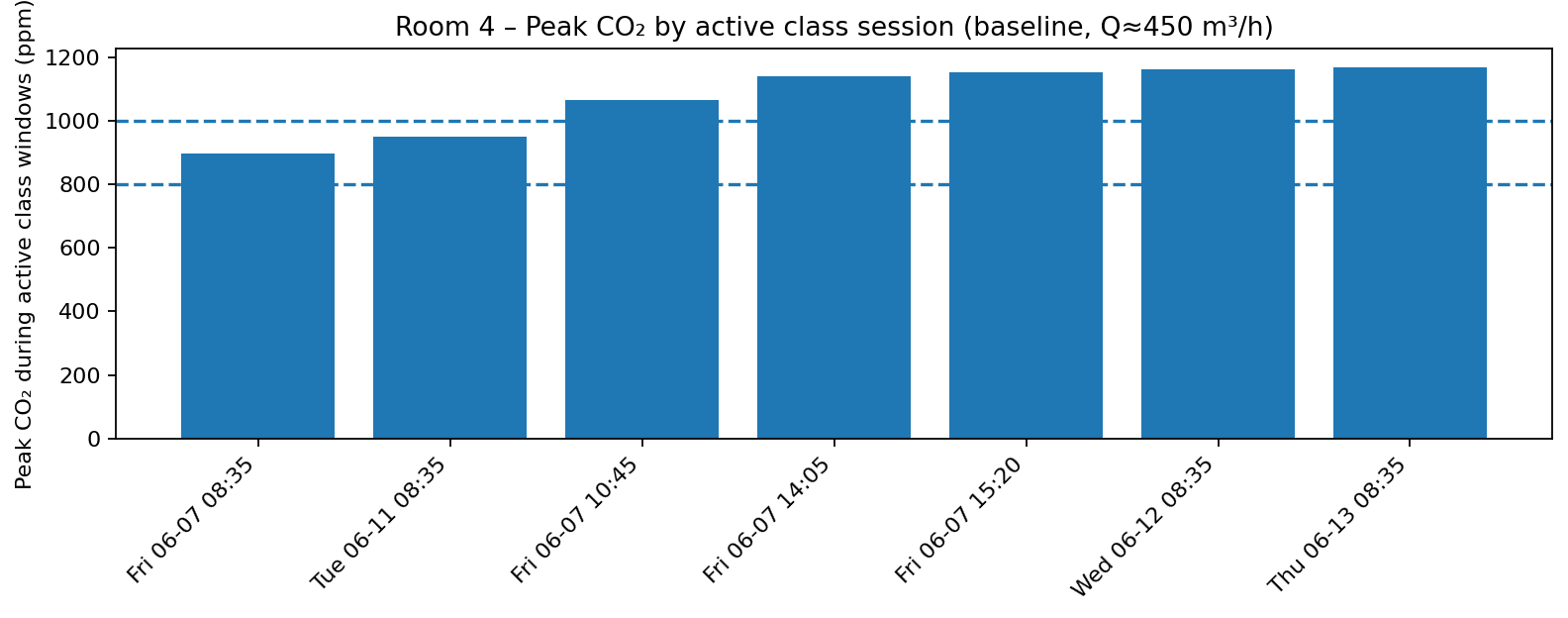
| Session start | Session end | Peak CO₂ (ppm) | Minutes >800 ppm | Minutes >1000 ppm | Average airflow (m³/h) |
|---|---|---|---|---|---|
| Thu 06-13 08:35 | 10:25 | 1168 | 90 | 70 | 428 |
| Wed 06-12 08:35 | 10:25 | 1162 | 85 | 60 | 431 |
| Fri 06-07 15:20 | 16:15 | 1153 | 100 | 95 | 450 |
| Fri 06-07 14:05 | 15:00 | 1141 | 40 | 25 | 441 |
| Fri 06-07 10:45 | 12:35 | 1066 | 110 | 75 | 446 |
| Tue 06-11 08:35 | 10:25 | 950 | 90 | 0 | 422 |
| Fri 06-07 08:35 | 09:30 | 897 | 25 | 0 | 409 |
Peak CO₂ is useful, but time above threshold is more revealing
Peak values are visually intuitive, but they do not tell the whole story. For commissioning and operations, the more revealing metric is often the amount of time spent above meaningful thresholds. In this review, two practical thresholds were used: 800 ppm and 1000 ppm.
Several sessions spend large periods above 800 ppm, and multiple sessions remain above 1000 ppm for a substantial portion of the analysed window. The window used here includes pre-ventilation, occupied time, and purge, which makes it useful for understanding the space’s ability to recover between occupancy periods rather than only its in-use average.
Figure 2. Time above 800 ppm and 1000 ppm during each active window in the case-study room
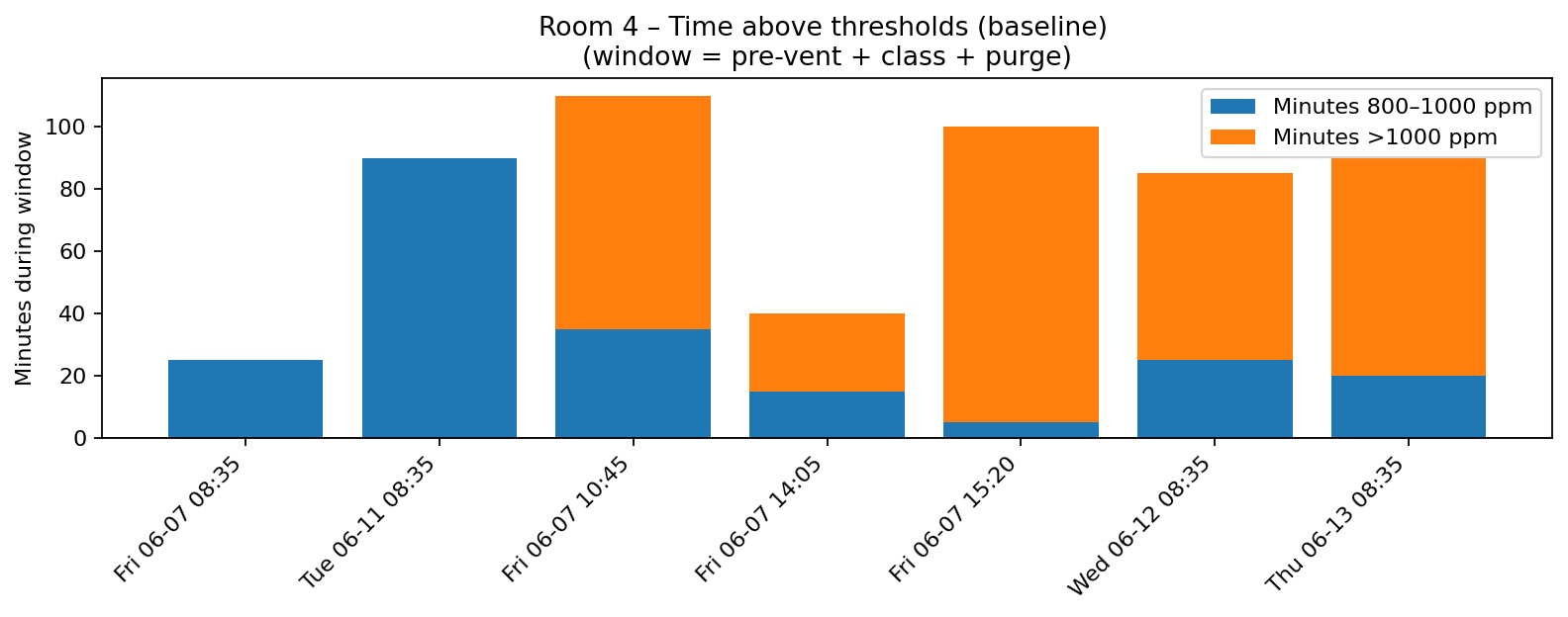
This is where one operational KPI becomes especially useful: CO₂ at the start of occupancy. If a new occupied period begins with already elevated CO₂, the space is effectively carrying a debt from the previous session. In those conditions, maintaining acceptable concentration becomes much harder unless the system delivers a meaningful boost early enough.
Why pre-ventilation alone is not enough
Pre-ventilation helps by lowering the starting concentration. That is valuable. But if the airflow during the occupied period itself remains close to the nominal baseline, long sessions can still drift above the target. Once the space is occupied and CO₂ generation continues, the system must either hold the concentration down during use or recover strongly enough during breaks to reset the space for the next occupancy period.
- Pre-ventilation helps the first part of occupancy.
- Reset or purge periods are critical to avoid cumulative carry-over.
- Long occupied periods still require sufficient in-use airflow capacity.
The real design question: are you targeting 1000 ppm or 800 ppm?
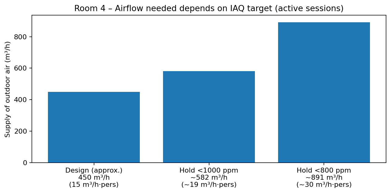
Using the measured dynamics and the calibrated mass-balance model, the estimated airflow requirements were as follows:
- To stay below about 1000 ppm: approximately 582 m³/h total outdoor airflow, or about 19 m³/h per person for 30 students
- To stay below about 800 ppm: approximately 891 m³/h total outdoor airflow, or about 30 m³/h per person
That difference is substantial. Holding the room below 800 ppm is not a small tuning adjustment relative to the baseline. It implies a significantly higher ventilation commitment.
Figure 3. Estimated outdoor airflow required for different IAQ targets in the case-study room
An 800 ppm target may be attractive from an IAQ perspective, but it creates a different system requirement in terms of fan headroom, duct pressure losses, terminal performance, and acoustic impact. A 1000 ppm target may be more achievable with moderate uplift plus better control, especially when capacity is constrained.
Can short purge bursts solve the problem?
The review also tested a practical operational idea: using a short, high-flow purge between occupied periods.
With a room volume around 130 m³, an initial concentration of 1100 ppm, and outdoor CO₂ at 400 ppm:
- 5 minutes at 450 m³/h would reduce concentration to about 925 ppm
- 5 minutes at 900 m³/h would reduce concentration to about 792 ppm
That corresponds to roughly 130 ppm of additional reset gained in just 5 minutes in that simplified case. But the assumptions matter. If the break is not a true break, if occupants remain in the room, or if the space returns immediately to low baseline airflow during the next long occupied period, the benefit is consumed quickly.
Indoor air quality data does not explain indoor air quality
This case study points to a broader issue in building performance work. In many projects, IAQ monitoring is presented as if it were the solution itself. Install sensors. Collect data. Build dashboards. But indoor air quality problems rarely come from a lack of data alone. They come from how the physical system is designed, controlled, maintained, and operated.
A sensor provides information, but it does not explain the system. A CO₂ sensor measures one point in space. The ventilation system may behave differently across the room. Airflow distribution depends on diffuser type, throw, induction, and supply velocity. Control performance depends on BMS logic, sensor location, reset strategy, and response time. Return measurements integrate the room with delay. That means the measured value is a consequence of system behaviour, not a direct explanation of the cause.
A graph can show that CO₂ is high. A dashboard can show that a threshold was exceeded. A trend can show that the room improved after a purge period. But none of those signals, on their own, tells us whether the root cause sits in the outdoor air path, the filter pressure loss, the fan head, the VFD logic, the static pressure strategy, the duct resistance, the terminal distribution, the mixing conditions in the room, or the actual control sequence implemented in the BMS.
- outdoor air intake conditions and location
- filter condition and pressure drop
- fan capacity, available static pressure, and VFD behaviour
- duct resistance and balancing condition
- diffuser design, air distribution, and room mixing
- BMS sequence of operations, sensor placement, and control logic
- real delivered outdoor airflow under occupied conditions
The same limitation applies to analytical models. Something happens in the real world. Only part of it becomes observable. Only part of that is measured. Only part of that becomes recorded data. The model then learns from that filtered version of reality. This is why a model can look mathematically convincing while still missing how the physical system truly behaves in operation.
For BAARCH, that is the critical engineering position. Monitoring is one layer of observation. It tells us whether performance appears good, average, or poor. But solving IAQ issues requires understanding the ventilation system itself: airflow, fan curves, control logic, delivered outdoor air, and actual room behaviour. In buildings, data is not the system. It is only a trace of how the system behaved.
Conclusion
Indoor air quality in commercial buildings is not only a matter of nominal ventilation rates. It is a matter of dynamics, reset quality, sensor interpretation, airflow delivery, and control strategy. A space can look acceptable from a design spreadsheet and still underperform in daily use when occupied periods are long, consecutive, and poorly reset between cycles.
The broader lesson is equally important. IAQ data does not explain IAQ by itself. It shows the outcome of how a physical system behaved. To understand why performance is good or poor, the engineering chain must be read as a whole: intake, fan, filter, pressure, control logic, air distribution, mixing, and delivered outdoor air. In classrooms, offices, retail spaces, meeting rooms, and many other commercial settings, the path to better air quality is rarely a single threshold or a more elegant dashboard. It is an engineered response grounded in physics, commissioning, and operational understanding.